Values such as inventory and balance account, usually calculated from a snapshot table, require the use of semi-additive measures. In Multidimensional you have specific aggregation types, like LastChild and LastNonEmpty. In PowerPivot and Tabular you use DAX, which is flexible enough to implement any calculation as described in this article.
UPDATE 2020-11-10: You can find more complete detailed and optimized examples (with both Power Pivot and Power BI files) for semi-additive calculations in the DAX Patterns: Semi-additive calculations article+video on daxpatterns.com.
UPDATE 2014-02-03: fixed errors in ClosingNonBlank functions thanks to Franj Tonsen’s comment.
A semi-additive measure does not aggregate data over all attributes like a regular additive measure would. For example, measures like balance account and product inventory units can be aggregated over any attribute but time. Instead of considering the time period selected (one year, one month …) you only consider a particular moment in time related to the time period selected. It could be the first day, the last day, the last day that had transactions, and so on.
This condition is typical for tables containing snapshots over time such as products inventory or accounts balances. In the following table, you can see an excerpt of a Product Inventory table. The same product has a Units Balance value for each date. Yet you cannot sum this column for two different dates, for example to calculate an average over different dates. If you want to calculate the value of Units Balance for July 2005, you need to filter the row for the last day of that month, ignoring rows for all the other days. However, you have to use a regular aggregation for other measures such as Units In and Units Out, which are regular additive measures.
| Product Name | Date Key | Units In | Units Out | Units Balance |
| … | … | … | … | … |
| Road-650 Red, 44 | 20050630 | 0 | 0 | 170 |
| Road-650 Red, 44 | 20050701 | 0 | 103 | 67 |
| Road-650 Red, 44 | 20050702 | 102 | 0 | 169 |
| Road-650 Red, 62 | 20050630 | 0 | 0 | 185 |
| Road-650 Red, 62 | 20050701 | 0 | 135 | 50 |
| Road-650 Red, 62 | 20050702 | 129 | 0 | 179 |
| … | … | … | … | … |
In order to implement a semi-additive measure in DAX, you use a technique that is similar to the one used to compute aggregations and comparisons over time. You change the filter over the date in a CALCULATE statement, but in this case you limit the range of selected dates instead of extending it (like year-to-date) or moving it (like prior year).
First and Last Date
You can use LASTDATE to get the last day active in the current filter context, for a particular date column passed as an argument. The result is a table of one column and one value that you can use as a filter argument in a CALCULATE statement, as in the following definition:
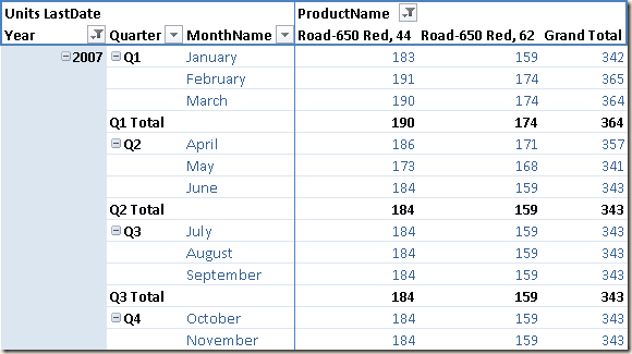
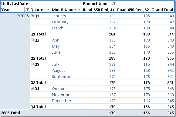
Units LastDate := CALCULATE ( SUM ( Inventory[UnitsBalance] ), LASTDATE ( 'Date'[Date] ) )
The result shows that the total for each quarter corresponds to the value of the last month in the quarter. For example, the Q1 value is the same as March. Each month value corresponds to the value of the last day in that month, not represented here.
First and Last Non Blank
The Units LastDate calculation assumes that there are data for every year in every month. If the inventory is daily, this is not an issue. However, it could become a problem if the inventory is written only for working days: if a month were to end on a Saturday, you would see the entire month. The problem is evident for future dates. In the following picture you see what happens when using Units LastDate with an Inventory table whose rows only go until December 15, 2007: you do not see the total for year 2007, for Q4, and for December!
The reason is that the LASTDATE formula operates on dates available in the filter context; also, the Date table contains all the days for the year 2007. This is a best practice, otherwise other Time Intelligence functions would not work correctly. You can use another DAX function, LASTNONBLANK, which returns the last date that satisfies a non-blank condition for an expression passed as second argument.
Units LastNonBlank :=
    CALCULATE (
        SUM ( Inventory[UnitsBalance] ),
        LASTNONBLANK (
            'Date'[Date],
            CALCULATE ( SUM ( Inventory[UnitsBalance] ) )
        )
    )
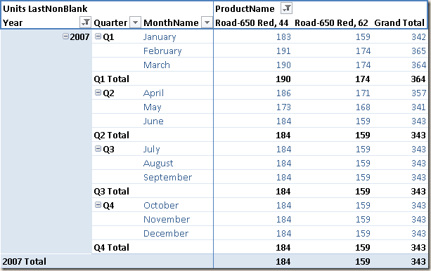
It is important that the second argument of the LASTNONBLANK apply the context transition using an implicit or explicit CALCULATE. Otherwise, you would apply the expression without filtering by each date in the time period, and the result would be identical to LASTDATE. You can see the result in the following picture, where December, Q4 and the total for 2007 are all displayed.
If you need the first date of a time period instead of the last date, you can use FIRSTDATE. You also have FIRSTNONBLANK to get the first date with any data, similar to what you do with LASTNONBLANK for the last date with any data. All these functions return a table of one column and one row: for this reason, you can use them in a filter argument of a CALCULATE call. A common mistake is assuming that LASTDATE and MAX would produce the same result. While this is true from a logical point of view, there is an important syntactic difference. You cannot write the following expression:
Units MaxDate :=
    CALCULATE (
        SUM ( Inventory[UnitsBalance] ),
        MAX ( 'Date'[Date] )
    )
The MAX function returns a scalar value, and the filter argument of a CALCULATE function requires a table expression or a logical condition referencing only one column. Thus, you use MAX instead of LASTDATE as in the following definition:
Units MaxDate :=
    CALCULATE (
        SUM ( Inventory[UnitsBalance] ),
        FILTER (
            ALL( 'Date'[Date] ),
            'Date'[Date] = MAX ( 'Date'[Date] )
        )
    )
You can also simplify the syntax by storing the MAX value in a variable, so you can use the shorter predicate condition in the CALCULATE argument.
Units MaxDate :=
    VAR LastDayInSelection = MAX ( 'Date'[Date] )
    RETURN CALCULATE (
        SUM ( Inventory[UnitsBalance] ),
        'Date'[Date] = LastDayInSelection
    )
The best practice is using LASTDATE when you write a filter expression, whereas MAX is better when you are writing a logical expression in a row context. This is because LASTDATE implies a context transition that hides the external filter context.
Opening and Closing Time Periods
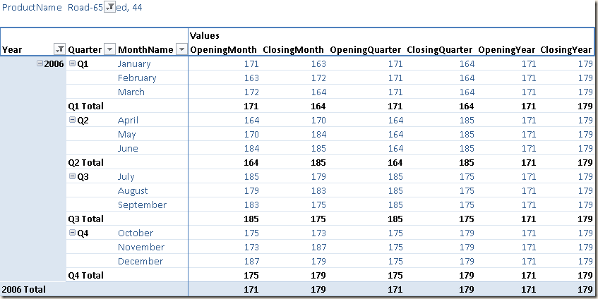
Other Time Intelligence functions are useful in semi-additive measures, for getting the first and last date of a period (year, quarter, or month). These are helpful whenever you need to extract a value of a selection that is smaller than the entire period considered. For example, looking at the month level which may be displayed in rows, you might want to also display the quarter end and year end values in that same row. You can see this in the following picture.
The definitions of the ClosingMonth, ClosingQuarter, ClosingYear, OpeningMonth, OpeningQuarter and OpeningYear measures used in the previous pivot table are the following:
ClosingMonth := CLOSINGBALANCEMONTH ( SUM ( Inventory[UnitsBalance] ), 'Date'[Date]  )
ClosingQuarter := CLOSINGBALANCEQUARTER ( SUM ( Inventory[UnitsBalance] ), 'Date'[Date]  )
ClosingYear := CLOSINGBALANCEYEAR ( SUM ( Inventory[UnitsBalance] ), 'Date'[Date]  )
OpeningMonth := OPENINGBALANCEMONTH ( SUM ( Inventory[UnitsBalance] ), 'Date'[Date]  )
OpeningQuarter := OPENINGBALANCEQUARTER ( SUM ( Inventory[UnitsBalance] ), 'Date'[Date]  )
OpeningYear := OPENINGBALANCEYEAR ( SUM ( Inventory[UnitsBalance] ), 'Date'[Date]  )
The previous measures correspond to the following ones defined using CALCULATE and using the filter provided by the ENDOFMONTH, ENDOFQUARTER, ENDOFYEAR, STARTOFMONTH, STARTOFQUARTER and STARTOFYEAR functions, respectively:
ClosingEOM := CALCULATE ( SUM ( Inventory[UnitsBalance] ), ENDOFMONTH ( 'Date'[Date] ) )
ClosingEOQ := CALCULATE ( SUM ( Inventory[UnitsBalance] ), ENDOFQUARTER ( 'Date'[Date] ) )
ClosingEOY := CALCULATE ( SUM ( Inventory[UnitsBalance] ), ENDOFYEAR ( 'Date'[Date] ) )

StartingSOM :=
CALCULATE (
    SUM ( Inventory[UnitsBalance] ),
    DATEADD ( STARTOFMONTH ( 'Date'[Date] ), -1, DAY )
)

StartingSOQ :=
CALCULATE (
    SUM ( Inventory[UnitsBalance] ),
    DATEADD ( STARTOFQUARTER ( 'Date'[Date] ), -1, DAY )
)

StartingSOY :=
CALCULATE (
    SUM ( Inventory[UnitsBalance] ),
    DATEADD ( STARTOFYEAR ( 'Date'[Date] ), -1, DAY )
)
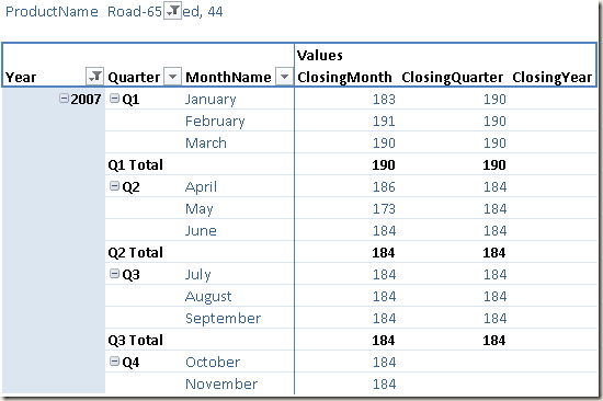
No functions for opening and closing periods consider the non-blank condition. You can see the behavior of the previous closing measures for the year 2007, where data is only available until December 15, in the following picture.
Instead of the OPENING/CLOSING functions, you should use the LASTNONBLANK function as filter in a CALCULATE statement, applying an extension of the time period considered using the PARALLELPERIOD function. Here are the corresponding definitions:
OpeningMonthNonBlank :=
    CALCULATE (
        SUM ( Inventory[UnitsBalance] ),
        CALCULATETABLE (
            LASTNONBLANK ( 'Date'[Date], CALCULATE ( SUM ( Inventory[UnitsBalance] ) ) ),
            PARALLELPERIOD ( 'Date'[Date], -1, MONTH )
        )
    )

OpeningQuarterNonBlank :=
    CALCULATE (
        SUM ( Inventory[UnitsBalance] ),
        CALCULATETABLE (
            LASTNONBLANK ( 'Date'[Date], CALCULATE ( SUM ( Inventory[UnitsBalance] ) ) ),
            PARALLELPERIOD ( 'Date'[Date], -1, QUARTER )
        )
    )

OpeningYearNonBlank :=
    CALCULATE (
        SUM ( Inventory[UnitsBalance] ),
        CALCULATETABLE (
            LASTNONBLANK ( 'Date'[Date], CALCULATE ( SUM ( Inventory[UnitsBalance] ) ) ),
            PARALLELPERIOD ( 'Date'[Date], -1, YEAR )
        )
    )

ClosingMonthNonBlank :=
    CALCULATE (
        SUM ( Inventory[UnitsBalance] ),
        CALCULATETABLE (
            LASTNONBLANK ( 'Date'[Date], CALCULATE ( SUM ( Inventory[UnitsBalance] ) ) ),
            PARALLELPERIOD ( 'Date'[Date], 0, MONTH )
        )
    )

ClosingQuarterNonBlank :=
    CALCULATE (
        SUM ( Inventory[UnitsBalance] ),
        CALCULATETABLE (
            LASTNONBLANK ( 'Date'[Date], CALCULATE ( SUM ( Inventory[UnitsBalance] ) ) ),
            PARALLELPERIOD ( 'Date'[Date], 0, QUARTER )
        )
    )

ClosingYearNonBlank :=
    CALCULATE (
        SUM ( Inventory[UnitsBalance] ),
        CALCULATETABLE (
            LASTNONBLANK ( 'Date'[Date], CALCULATE ( SUM ( Inventory[UnitsBalance] ) ) ),
            PARALLELPERIOD ( 'Date'[Date], 0, YEAR )
        )
    )
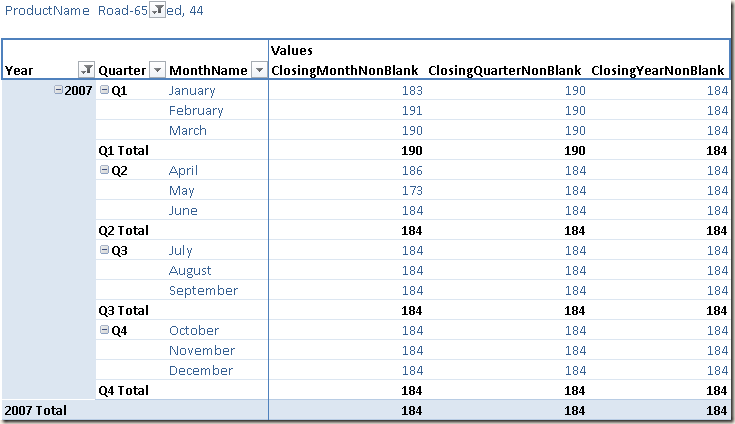
The following is the final result using these measures for the year 2007.
The filter calculation might be different according to the logic you want to implement, but the pattern for a semi-additive measure is to filter a single date based on the initial selection of dates in the filter context. This logic is usually in a filter argument of a CALCULATE function call – unless a special time intelligence function is used, hiding the internal calculation that is always applied on a CALCULATE statement.
You can hear me explain a few aspects of semi-additive measures in the DAX Time Intelligence video.
