You can implement the calculation of stock inventory over time in several ways in DAX. The xVelocity technology in Power Pivot and Analysis Services Tabular is so fast that you might considerboth dynamic calculation and snapshot based calculation,depending on volume and distribution of data.

When you want to analyze stock inventory over time, the traditional approach is creating an Inventory table that contains, for every day, the quantity for every product that is in stock. Such a table makes it very quick retrieving the stock amount of one or more products, because you have to sum only the rows for a single day. The Inventory table is also known as a “snapshot” table, which means that for every day you have a complete description of the stock availability. There should be some batch processing (usually part of the ETL nightly process) that updates this table every day and the size of this table increase every day by the number of products available, assuming you do not store a row for products that are out of stock.

The size of an Inventory table might be huge. A business that everyday has a large amount of transactions for most of the products in stock would prefer using the Inventory table, because it is smaller than the Movements one. However, if a business has many products available in stock and most of them do not have movements every day, then the Inventory table might have a size that is a multiple of the Movements table.

In Power Pivot and Analysis Services Tabular, all data is stored in memory. Even if the high compression ratio reduces the size of the table, the Inventory storage might be expensive and you can avoid this snapshot table by calculating the Units In Stock value dynamically at query time. The tradeoff between memory cost and query speed depends on many factor and you have to evaluate when this technique is affordable on a case-by-case basis.

You can download two sample workbooks: one (Warehouse Stock – Inventory) extracts the inventory fact table from AdventureWorksDW2012 sample database. The following is the schema of the data model.

The other (Warehouse Stock – Movements) has a query that generates the corresponding Movements table, generating one row for each in and out transaction. You will see up to two rows for each product every day. The schema of the data model is similar, the difference is in the calculation we have to implement.

DAX Calculation

The DAX formula using the Inventory table simply filters the last date available in the selected period.

UnitsInStock :=
CALCULATE ( 
    SUM ( Inventory[UnitsBalance] ),
    LASTDATE ( 'Date'[Date] )
)

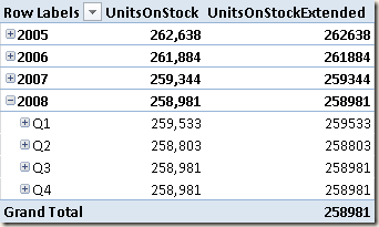
You might prefer using LASTNONBLANK instead of LASTDATE:

UnitsInStockExtended:=CALCULATE ( 
    SUM ( Inventory[UnitsBalance] ),
    LASTNONBLANK ( 'Date'[Date], CALCULATE ( SUM ( Inventory[UnitsBalance] ) ) )
)

In case you do not have the inventory already evaluated for all the days in one year, the UnitsInStockExtended calculation propagates the last inventory in the following days. Since the Inventory we used already has transactions for all the days in the last year available, you can see the difference between the two measures only at the Grand Total level.

The alternative approach requires the calculation of all the Movements with a date that is less than or equal to the date of the inventory you want to consider. In other words, you apply a CALCULATE function that is similar to the one used for a running total over dates, as you see in UnitsInStockSimple definition:

UnitsInStockSimple :=
CALCULATE ( 
    SUM ( Movements[Quantity] ),
    FILTER (
        ALL ( 'Date'[Date] ),
        'Date'[Date] <= MAX( 'Date'[Date] )
    )
)

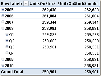
The simple formula you have seen propagates the last value to all the following days, regardless of the fact that there are no more transactions available. You can avoid this propagation by adding an IF statement that checks whether the period selected has some transactions in the Movements table.

UnitsInStock :=
IF ( 
    MIN ( 'Date'[DateKey] ) <= CALCULATE ( MAX ( Movements[DateKey] ), ALL ( Movements ) ),
    CALCULATE ( 
        SUM ( Movements[Quantity] ),
        FILTER (
            ALL( 'Date'[Date] ),
            'Date'[Date] <= MAX ( 'Date'[Date] )
        )
    )
)

You can see that the UnitsInStock measure does not produce a result for years and quarters in which there are no transactions.

Performance Considerations

The two
workbooks have a different size and a different number of rows in the table
containing the measures.

The Movements table has only 4.8% of the rows of the Inventory table, but it is 21% is size. This is because data in Inventory has many duplicates, which improve the compression ratio. These numbers might vary depending on the data distribution, so you should always consider that before making any decision. In this example, there are 606 products, but only 276 products have a transaction other than the initial balance. There are 1126 days with at least one transaction. There is an average of 32.8 transactions per day and every product that has some movement has a transaction every 8.5 days.

A comparison made using three different DAX queries returning the same data from the two data models produces many interesting information.

The engine evaluates the stock measure for every row in the result. You can assume that every cell in a PivotTable corresponds to an execution, so the query corresponds to a PivotTable with 2500 rows and 12 columns. The dynamic calculation using Movements is slower than the snapshot-based model using Inventory when the number of rows returned is small. However, with a higher number of rows returned there is a strange effect that makes the dynamic calculation faster. In this case, the snapshot pattern is faster only for queries that executes in less than one second, but for longer queries the dynamic calculation performs much better.

You can see the queries used below: just replace Movements with Inventory in order to execute the queries on the snapshot-based data model.

Query A

EVALUATE
ADDCOLUMNS (
    SUMMARIZE (
        Movements,
        'Date'[Date],
        'Products'[Category]
    ),
    "UnitsInStock", [UnitsInStock]
)
ORDER BY 'Date'[Date],
         'Products'[Category]

Query B

EVALUATE
ADDCOLUMNS (
    SUMMARIZE (
        Movements,
        'Date'[Year],
        'Date'[Month],
        'Products'[Category]
    ),
    "UnitsInStock", [UnitsInStock]
)
ORDER BY
        'Date'[Year],
        'Date'[Month],
        'Products'[Category]

Query C

EVALUATE
ADDCOLUMNS (
    SUMMARIZE (
        Movements,
        'Date'[Date],
        'Products'[ProductKey]
    ),
    "UnitsInStock", [UnitsInStock]
)
ORDER BY 'Date'[Date],
         'Products'[ProductKey]

Conclusion

Using the dynamic calculation for stock inventory seems a good idea because it allows a big space saving if most of the products do not have transactions every day. Generally, there is a performance penalty at query time by using the dynamic calculation, but it seems that this penalty might disappear on large result sets. We have observer better performance in dynamic calculation with a large result set, which could be the case of a chart displaying the stock level over time for different products. You should carefully test the performance and the space saving of dynamic calculation with your data before choosing to implement it in production.