This article describes the differences between eager evaluation and strict evaluation in DAX, empowering you to choose the best evaluation type for your data models.
A conditional expression in DAX – like an IF function – can be evaluated in two ways: eager and strict. Understanding the difference between the two evaluation modes can be very useful in finetuning the performance of a measure. The examples in this article cover strict and eager evaluation. The goal is to equip you to make an informed decision in picking the best evaluation mode for a specific data model.
The first example is a simple measure that performs a comparison and then returns one of two different values depending on the outcome of the comparison. Consider the following query:
EVALUATE
VAR AverageSales =
    [Sales Amount] / DISTINCTCOUNT ( 'Product'[Color] )
RETURN
    ADDCOLUMNS (
        VALUES ( 'Product'[Color] ),
        "@Test", IF (
            [Sales Amount] > AverageSales,
            [Margin],
            [Total Cost]
        )
    )
The @Test column contains either the Margin or the Total Cost result, depending on whether the Sales Amount of the given color is higher than the AverageSales per color or not. This is a useless calculation – we are not interested in the result, but rather in how the DAX engine computes it.
The engine starts by computing the AverageSales variable. Then, it has a choice. The first option is to compute the value of the condition at line 8 for each color – checking whether Sales Amount for the given color is larger than AverageSales – before computing either Margin or Total Cost, choosing to calculate only the one that is required by the result of the condition. This behavior is the most intuitive and it is known as strict evaluation in Analysis Services and Power BI. Another well-known name for this technique is short-circuit evaluation.
There is another way of computing the same result. The engine could compute every measure (Margin, Total Cost, and Sales Amount) for every product color. Once all these values are available, the engine would check the condition for each color and choose whether to use the previously computed value of Margin or Sales Amount. This technique is known as eager evaluation and consists in precomputing all the possible values that could be returned by a conditional statement, choosing which value to use case by case at a later time.
Which of the two techniques is better? You already know the answer: it depends. Though strict evaluation may look more efficient, this is not always the case. Before moving further, consider a simple example. What if the expression for the @Test column looked like this:
EVALUATE
VAR AverageSales =
    [Sales Amount] / DISTINCTCOUNT ( 'Product'[Color] )
RETURN
    ADDCOLUMNS (
        VALUES ( 'Product'[Color] ),
        "@Test", IF (
            [Sales Amount] > AverageSales,
            [Sales Amount] * 1.5,
            [Sales Amount] * 2.0
        )
    )
In this expression, the same sub-expression [Sales Amount] is used in both branches of the IF statement. Strict evaluation requires computing the Sales Amount measure once in order to determine which colors satisfy the condition; then the same Sales Amount measure is computed a second time to solve the expression chosen by the condition. In other words, the engine needs to scan the Sales table multiple times in order to obtain the results required.
By using eager evaluation, the DAX engine computes the value of Sales Amount for each color in a single scan; only later does it check the condition defining which of the two expression to return. This means that the eager evaluation requires fewer scans of the Sales table.
However, this does not mean that eager evaluation is always the best choice. It is better in the example outlined, but there are many scenarios where strict evaluation proves to be the best option. Nevertheless, since strict evaluation is intuitively better, we wanted to start with an example where eager evaluation is indeed the best option.
Let us elaborate more on the topic by looking at the actual query plan of the query described at the beginning of this article; it is reported in the following code snippet, which also includes the definition of the measures:
DEFINE
    MEASURE Sales[Margin] =
        SUMX (
            Sales,
            Sales[Quantity] * ( Sales[Net Price] - Sales[Unit Cost] )
        )
    MEASURE Sales[Sales Amount] =
        SUMX (
            Sales,
            Sales[Quantity] * Sales[Net Price]
        )
    MEASURE Sales[Total Cost] =
        SUMX (
            Sales,
            Sales[Quantity] * Sales[Unit Cost]
        )
EVALUATE
VAR AverageSales =
    [Sales Amount] / DISTINCTCOUNT ( 'Product'[Color] )
RETURN
    ADDCOLUMNS (
        VALUES ( 'Product'[Color] ),
        "@Test", IF (
            [Sales Amount] > AverageSales,
            [Margin],
            [Total Cost]
        )
    )
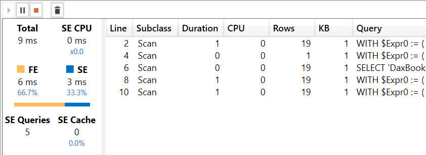
The DAX query generates five Storage Engine (SE) queries.

Two of these five queries are not interesting: one at line 4 is needed to compute AverageSales and one at line 6 is required to obtain the full list of the Product[Color] values. The other three queries are more interesting. Please note that all queries have been edited to make them easier to read.
The query at line 2 computes Sales Amount for every color. It is required to evaluate the condition for all the possible colors:
SELECT
    'Product'[Color],
    SUM ( 'Sales'[Quantity] * 'Sales'[Net Price] )
FROM 'Sales'
    LEFT OUTER JOIN 'Product' ON 'Sales'[ProductKey]='Product'[ProductKey]
The last two queries at line 8 and line 10 compute Margin and Total Cost respectively, for a different subset of colors. The DAX Formula Engine (FE) evaluates the condition for the colors using the result of the previous query, and then splits the colors into two lists: one list contains the colors returning true in the IF condition – computing Margin in that case – while the other list contains the colors returning false for the same IF condition – computing Total Cost as a result:
SELECT
    'Product'[Color],
    SUM ( 'Sales'[Quantity] * ( 'Sales'[Net Price] - 'Sales'[Product Cost] ) )
FROM 'Sales'
    LEFT OUTER JOIN 'Product' ON 'Sales'[ProductKey]='Product'[ProductKey]
WHERE
    'Product'[Color] IN ( 'Black', 'Silver', 'Blue', 'White', 'Grey' )

SELECT
    'Product'[Color],
    SUM ( 'Sales'[Quantity] * 'Sales'[Product Cost] )
FROM 'Sales'
    LEFT OUTER JOIN 'Product' ON 'Sales'[ProductKey]='Product'[ProductKey]
WHERE
    'Product'[Color] IN ( 'Red', 'Green', 'Orange', ..[11 total values, not all displayed] )
The engine does not compute the total cost for all the colors. Every color appears in only one of the two SE queries, depending on the condition evaluated for each color in the previous evaluation.
At this point we are curious to see the same query with eager evaluation. In order to enforce the eager evaluation, we change the code a bit by introducing variables:
EVALUATE
VAR AverageSales = [Sales Amount] / DISTINCTCOUNT ( 'Product'[Color] )
RETURN
    ADDCOLUMNS (
        VALUES ( 'Product'[Color] ),
        "@Test",
            VAR Margin = [Margin]
            VAR SalesAmount = [Sales Amount]
            VAR TotalCost = [Total Cost]
            RETURN
                IF (
                    SalesAmount > AverageSales,
                    Margin,
                    TotalCost
                )
    )
The values used inside the IF function are now computed before the IF, storing them into variables (Margin, SalesAmount, and TotalCost). We are explicitly telling the engine the execution path that we want: first, compute all the values for every color; then, choose the result between the values computed depending on a condition (SalesAmount > AverageSales). This way, DAX follows our request and uses eager evaluation.
This results in only three SE queries: two SE queries are identical to the first two described in the previous DAX query, because they are required to compute the list of colors and the AverageSales variable. The remaining SE query retrieves the values of the three Margin, Sales Amount, and Total Cost measures with a single request:
SELECT
	'Product'[Color],
	SUM ( 'Sales'[Quantity] * 'Sales'[Net Price] ),
	SUM ( 'Sales'[Quantity] * ( 'Sales'[Net Price] - 'Sales'[Product Cost] ) ),
	SUM ( 'Sales'[Quantity] * 'Sales'[Product Cost] )
FROM 'Sales'
	LEFT OUTER JOIN 'Product' ON 'Sales'[ProductKey]='Product'[ProductKey]
Once the three Margin, SalesAmount, and TotalCost variables are computed for every color, the FE iterates the result of this last SE query. It does so choosing for each color whether to use Margin or TotalCost, depending on the condition evaluated using the SalesAmount of the color and the AverageSales computed earlier.
For such simple queries, there is no difference in the overall execution times because they both stand well under 10 milliseconds. Nevertheless, on large queries and/or with complex measures, the difference might be very noticeable.
The main elements driving the choice between eager versus strict evaluation are the following:
- Complexity of the expressions depending on a condition (like in an IF function). If the expression in the alternative branches of execution is very complex, then strict evaluation should be preferred because it exclusively reduces the number of calculations to the required rows.
- Presence of common sub-expressions in the expressions depending on a condition. If the same sub-expression is used in alternative branches of execution, then eager evaluation lets the engine optimize the execution by computing the sub-expression only once. With strict evaluation, the sub-expression must be computed multiple times – once for each of the alternative branches of execution.
- Sparsity of the result. If the IF function does not have an else branch of execution and it filters , then a strict evaluation reduces the number of computations to only the ones required.
Trying to simplify: For simple calculations like SUMX aggregations using simple expressions or for non-selective conditions, the eager evaluation usually works better. For more complex calculations or for very selective conditions, then the strict evaluation is a better choice.
For educational reasons, the code outlined in this article is quite simple. For complex DAX measures or queries, a deeper evaluation is required before choosing one technique over the other.
As an example, in a previous article (Optimizing conditions involving blank values in DAX) we showed a query that could potentially iterate over 15 million combinations, 99 thousand of which actually returned a result.
Using strict evaluation on that query resulted in having to compute a table with all possible 25 million rows, just to evaluate the condition for all the possible combinations. In that article, we had established other considerations; but the bottom line is that the best possible optimization for that scenario is to use variables in order to force eager evaluation. By using eager evaluation, the engine aggressively computes all the required expressions with a single scan of the fact table. The result includes 99 thousand rows and the engine knows that none of the remaining combinations will return a useful result. Eager evaluation proved to really shine in that case.
As with any article about optimization, remember that we never provide golden rules. The choice of strict versus eager optimization is one of the many tools in the DAX guru’s toolbelt. Next time you write an IF function inside an iteration over a large table, you want to also consider whether you are resorting to a strict or an eager evaluation.
Remember: never make a choice without proper testing. The best formula for one model might not be the best formula for a different model.
Have fun with DAX!